A quick review of key concepts in digital signal processing such as aliasing, DFT, convolution, FIR/IIR filters, etc.

Aliasing

Waves at frequencies $f$ and $(f + k \cdot f_s)$ look identical when sampled at rate $f_s$.

If a signal $x$ has frequency content only within the $range \pm B$ Hz, then the sampling rate must be at least $f_s = 2B$ to avoid aliasing.

$f_s/2$ is called the Nyquist frequency (for sampling rate $f_s$)

Fourier transform

DFT (Discrete Fourier transform)

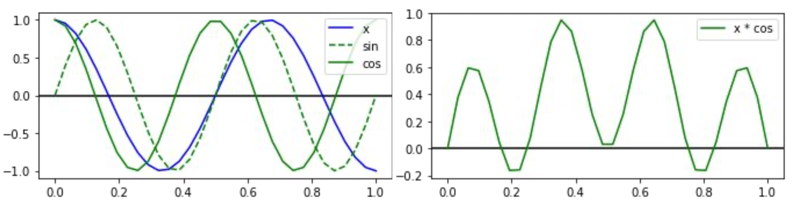
Intuition: cross-correlate the signal against cosine and sine waves of different frequencies.

$$ X[m] = \sum_{n=0}^{N-1} x[n] \cdot (cos(2 \pi \cdot m \cdot n / N) - j \cdot sin(2 \pi \cdot m \cdot n / N)), m \in [0, N-1] $$

With Euler’s formula:

$$ X[m] = \sum_{n=0}^{N-1} x[n] \cdot e^{-j2 \pi \cdot m \cdot n / N} $$

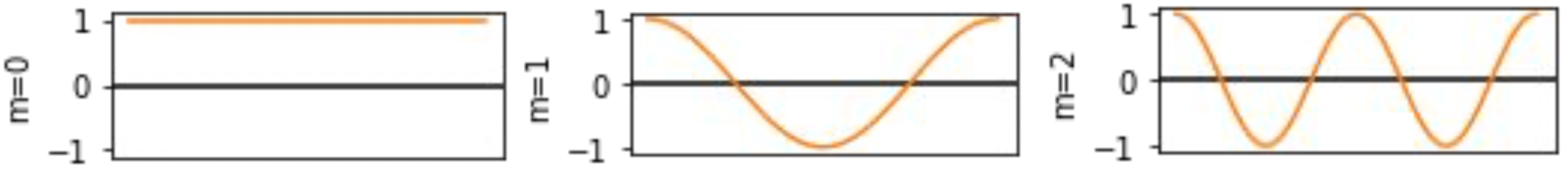
$m^{th}$ analysis frequency has exactly $m$ cycles over the duration of the signal $N$, and $f_m = m \cdot f_s / N$ HZ. The gap between $f_m$ and $f_{m+1}$ is called the bin spacing

DFT symmetry

For real valued $x[n]$,

$$e^{-j \cdot 2 \pi \cdot (N-m) \cdot / N} = e^{+j \cdot 2 \pi \cdot m \cdot m / N}$$

In other words, $X[m] = X^{*}[N-m]$, or frequencies $N/2+1, …, N-1$ are conjugates of $N/2-1, …, 1$ (identical real parts, reverded-signed imaginary parts)

DFT properties

Shifting

If $x_2[n] = x_1[n-D]$, then $X_2[m] = X_1[m] \cdot e^{-j2 \pi \cdot m \cdot D/N}$

• Derivation:

1. $|X_1[m]| = |X_2[m]|$
2. for $x(t) = cos(2 \pi \cdot f_0 \cdot t - \varphi)$, phase offset in the DFT is $e^{-j \varphi}$
3. if $D < N$, then $D/N$ is the proportion of entire signal being delayed, and $X_2[m]$ rotates $m$ times by angle $-2 \pi \cdot D/N$

Linearity

$$ \sum_{n} (c_1 \cdot x_1[n] + c_2 \cdot x_2[n]) \cdot e^{-j2 \pi \cdot m \cdot n / N} = c_1 \cdot X_1[m] + c_2 \cdot X_2[m] $$

In other words, scale and sum in time domain is equivalent to scale and sum in frequency domain

Combining linearity and shifting

$$ x[n]= \sum_k A_k e^{-2 \pi \cdot k \cdot n/N - \varphi_k} \Rightarrow X[m] = A_m e^{-j \varphi_m} $$

• when $k = m$, $e^{j2 \pi \cdot (k-m) \cdot n/N} = e^0 = 1$, thus
  $$X[m] = A_m e^{-j \varphi_k}$$
• when $k$ ≠ $m$, the summation over all $n$ cancels out, thus
  $$X[m] = 0$$

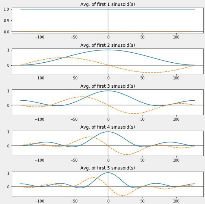
IDFT (Inverse DFT)

$$ x[n] = 1/N \cdot \sum_m X[m] \cdot e^{+j2 \pi \cdot m \cdot n/N} $$

For each term $X[m] \cdot e^{+j2 \pi \cdot m \cdot n/N} = A \cdot e^{j(j \pi \cdot m \cdot n/N + \theta)}$, which is a complex sinusoid with amplitude $A$, phase $\theta$, and frequency $mf_s/N$ [Hz] (or $m$ [cycles per signal duration]). In other words, every signal can be expressed as a weighted sum of sinusoids

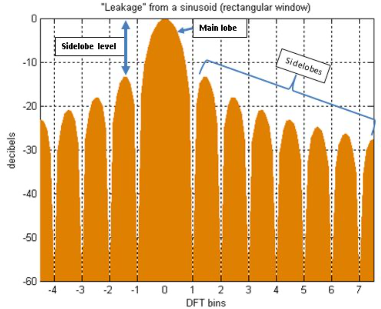
Spectral leakage

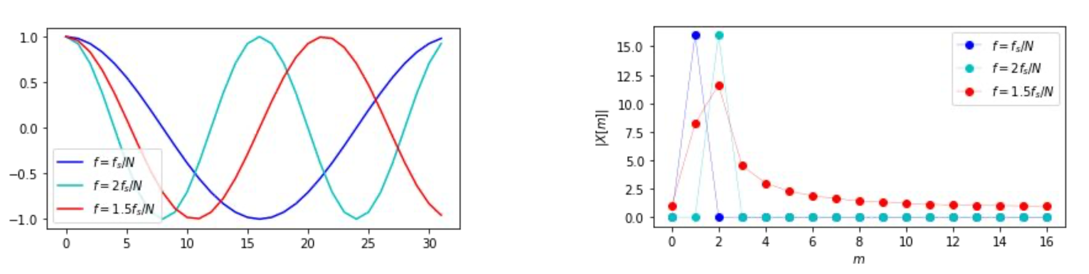
If a digital signal $x[n]$ has energy at frequencies which are not integer multiples of $f_s/N$, then this energy will leak (spread) across multiple DFT frequency bands $X[m]$

This is caused because such frequencies don’t have the whole number of cycles during sampling duration, so comparing to an analisis frequency won’t cancel out.

In this situation, $X[m]$ measures not just energy associated with the $m^{th}$ analysis frequency, but has contributions from every other non-analysis frequency.

Leakage compensation

Strategy #1: Have large N

Long signals, high sampling rate $\Rightarrow$ more analysis frequencies, smaller gaps between them

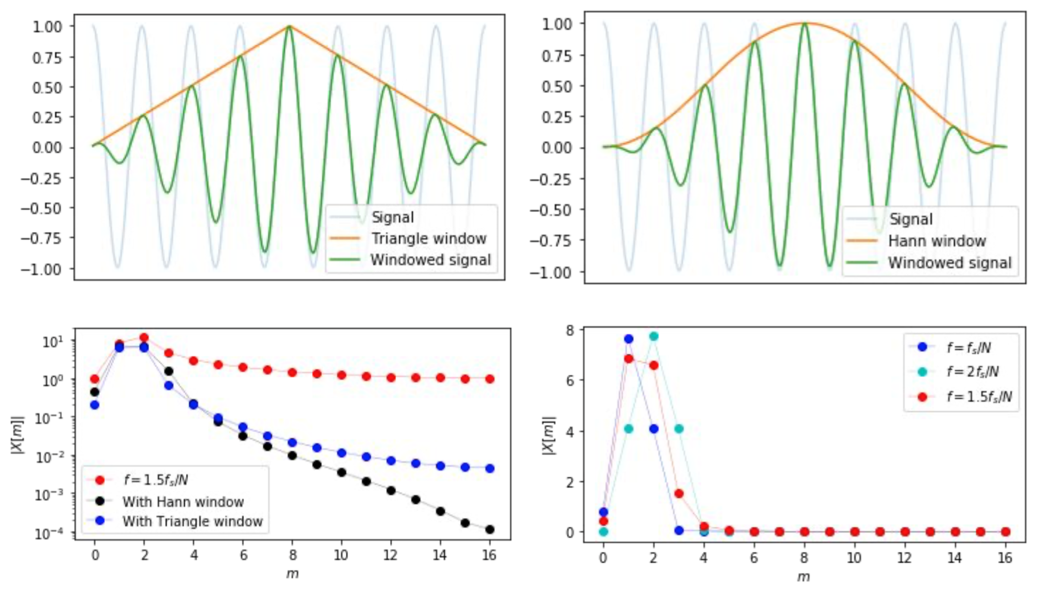
Strategy #2: Windowing

Intuition: force continuity at the edges, eliminate fractional cycles

Before taking the DFT, Multiply $x[n]$ by a window, which tapers the ends of the signal to (near) 0:
$$ x[n] \rightarrow w[n] \cdot x[n] $$

Result: leakage concentrates on nearby frequencies, and is reduced for distant frequencies; at the same time, analysis frequencies leak to their neighbors as well:

Since in naturally occurring signals, pure tones at exactly $mf_s/N$ hardly happen, we are unlikely to tell apart analysis and non-analysis frequencies. The overall benefits of windowing outweigh the drawbacks

Key properties when designing/choosing a window:

1. Width of the main lobe(in Hz or bins): how far does energy smear out locally
2. Hight of the side lobe(in dB): how loud is the leakage from distant frequencies

STFT(short-time Fourier transform)

Process

1. Carve the signal into small frames, with frame length $K$ and hop length $h$:
   • x[0], x[1], …, x[K-1]
   • x[h], x[h+1], …, x[h+K-1]
   • x[2h], x[2h+1], …, x[2h+K-1]
   • …
2. Window each frame to reduces leakage and artifacts from frame slicing
3. Compute the DFT of each windowed frame

Parameters & design

• Longer window (larger frame length $K$) means:
  • lower frequencies ($f_{min} = f_s / K$)
  • higher frequency resolution ($f_{max}$ is determined by Nyquist, number of analysis frequencies depends on frame length)
  • more data, more memory and compute
• $K$ with value of power of 2 (512, 1024, …) is ideal for FFT, pick $K$ to give the desired frequency resolution
• Smaller hop (smaller hop length $h$) means:
  • higher temporal resolution
  • more data, more memory and compute
• $h < K$, usually set hop = $K/2$ or $K/4$

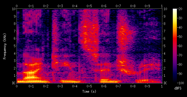
Spectrogram

A spectrogram is the STFT as an image, with each column as DFT of one frame into magnitude, which is usually log-scaled to decibels (dB). $log_2$ preserves visual size of octaves.

$$ X[m] \rightarrow 20 \cdot log_{10}|X[m]| [dB] $$

FFT (Fast Fourier Transform)

Idea: identify redundant calculations shared betwen different analysis frequencies, reducing time complexity from $O(N^2)$ to $O(N \cdot log(N))$

• FFT computes the DFT
• Requires signal length to be the power of 2 (1024, 2048, etc); otherwise pad up signal to the next power of 2 length
• FFT could be further optimized when the input is real-valued (the rfft() function in most FFT libraries) by taking use of conjugate symmetry

Convolution

Definition

$$ y[n] = \sum_{k=0}^{K-1}h[k] \cdot x[n-k] = x * h $$

$h$ is filter coefficients ordered from most recent ($h[0]$) to least recent ($h[K-1]$), while $x$ is ordered by increasing time $ \Rightarrow $ reversing $x$ to line up with $h$

Modes

1. Valid: no zero-padding, $[N]*[K] \rightarrow [N-K+1]$
2. Same: zero-padding before the signal, $[N]*[K] \rightarrow [max(N, K)]$
3. Full: pad by zeros on both ends, $[N]*[K] \rightarrow [N+K-1]$
4. Circular: like Same mode except $x$ is looped instead of zero-padded

Simple filters

• Gain: $h=[G]$
  • $x[n] \rightarrow G \cdot x[n]$
• Delay: $h=[0, 0,…, 1]$
  • $x[n] \rightarrow x[n+d]$
• Averaging: $h=[1/K, 1/K,…, 1/K]$
  • fast changes get smoothed out, making a crude low-pass filter
• Differencing: $h=[1, -1]$
  • crude hight-pass filter

Property

1. Linearity: $(c_1x_1+c_2x_2)h = c_1x1h+c_2x_2*h$
2. Commutativity: $xh = hx$ (we can treat the signal as the filter)
3. Associativity: $(xh)g = x(hg)$

Similar to wave propagation, where after reflection the signal gets delayed and attenuated, and microphone sums up the waves from both direct path as well as reflection path, each $x[n-k]$ could be regarded as being

1. delayed by $k$ time steps
2. scaled by $h[k]$
3. added together

Since convolution is linear and time invariant, every LSI system can be expressed as a convolution, and the “filter” $h$ is the impulse response of the system, which completely determines the behavior of the system.

If $h$ is finite in length, it’s called a Finite Impulse Response(FIR)

Convolution theorem

Convolution (int circular mode¹) in the time domain $x*h$ $\Leftrightarrow$ multiplication in the frequency domain $X \cdot H$, or

$$ DFT(x*h) = DFT(x) \cdot DFT(h) $$

Fast convolution

• Convolution in time domain has a time complexity of $O(N \cdot K)$
• In the frequency domain, it takes $N$ multiplies, so
  1. zero-pad $h$ from $K$ to $N$ samples
  2. compute two forward DFTs $O(2 \cdot N \cdot log_2N)$
  3. compute one inverse DFT $O(N \cdot log_2N)$
  4. totally $O(N \cdot log_2N)$

Filters

Frequency domain is complex-valued, with multiplication rule:

$$ (r \cdot e^{j \theta}) (s \cdot e^{j \varphi }) = (r \cdot s) \cdot e^{j(\theta + \varphi)} $$

FIR filters

Finite Impulse Response means the system’s response to an impulse goes to 0 at finite time step, or $y[n]$ depends on finitely many inputs $x[n-k]$.

• Positives:
  • Usually more simple to implement
  • can analyze by DFT
  • stable and well-behaved
• Negatives:
  • may not be efficient
  • somewhat limited expressivity (non-adaptive)

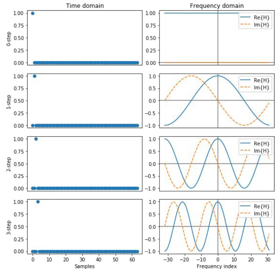
Delayed impulse analysis

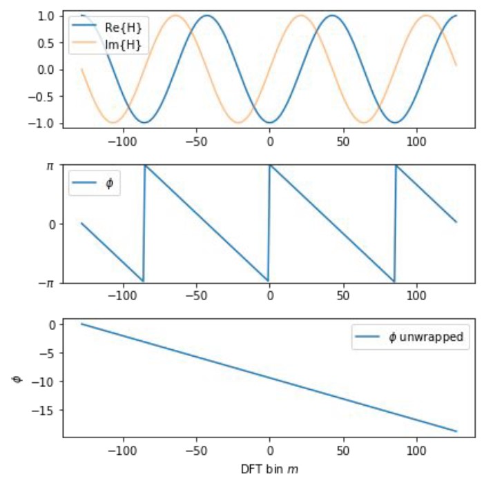
A k-step delay filter $h_k = [0, 0, 0, …, 1]$ has DFT $H_k[m]=e^{-j2 \pi \cdot m \cdot k/N}$, which is a sinusoid of frequency $k$.

Phase response of a delay filter (wrapped & unrapped):

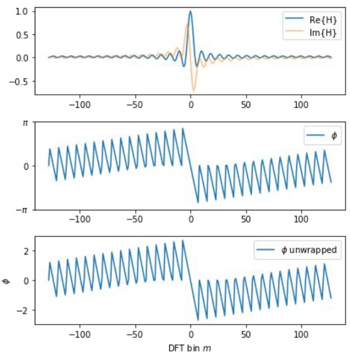
Averaging filter (rectangle/box) analysis

K-tap averaging filter $h_a = [1/K, 1/K, …, 1/K, 0, 0, …]$, which could be regarded as an average of K delayed filters. Thus,
$$ H_a[m] = DFT(h_a) = 1/K \sum_k DFT(h_k)[m] = 1/K \sum_k e^{-j2 \pi \cdot m \cdot k/N} $$

The real part $Re{H_a}$ is a $sinc$ function. If we apply $h_a$ to input signal $x$, according to convolution theorem, we multiply them in frequency domain, and magnitudes of output is: $|X[m] \cdot H[m]| = |X[m]| \cdot |H_a[m]|$. Since $|H_a[m]|$ decays slowly but bounces up and down in high frequency, there will be high frequency components remaining if we use averaging filter as a low pass filter.

Phase response of a rectangle filter is sawtoothy even after unwrapping, but it’s ok since it’s linear within the pass-bands:

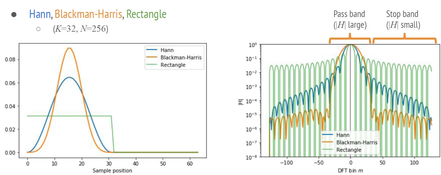
Typical FIR window analysis

Most window functions for DFT could be used as low-pass filters. Below is the frequency response for Hann, Blackman-Harris, and Rectangle window.

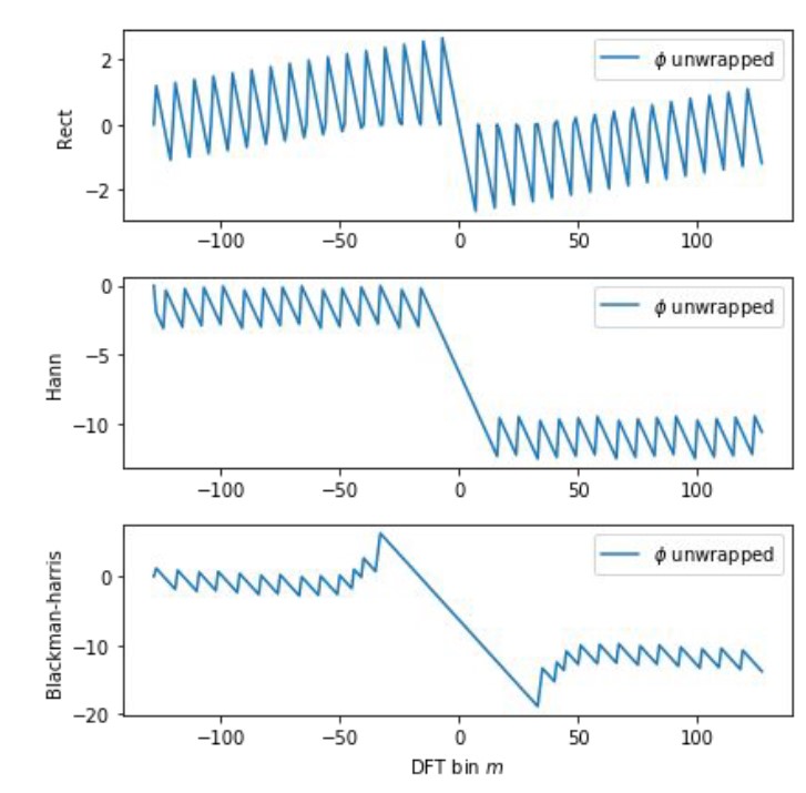
Since the windows above are linear within the pass-bands, audible frequencies will have constant delay without noticeable phasing artifacts:

IIR filters

Infinite Impulse Response filters can depend on infinitely many previous inputs by feedback:

$$ y[n] = \sum_{k=0}^K b[k] \cdot x[n-k] - \sum_{k=1}^K a[k] \cdot y[n-k] $$

Here $K$ is the order of the filter. If we define $a[0] = 1$, then we get:

$$ \sum_{k \geq 0} a[k] \cdot y[n-k] = \sum_{k \geq 0} b[k] \cdot x[n-k] $$

Due to the feedback, to achieve comparable results, IIR filters need fewer coefficients and multiply-adds with lower latency than FIR filters, so it can be much more efficient.

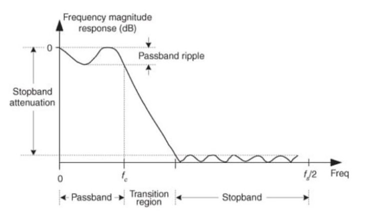
To analyze frequency response of filters, we usually use following parameters to measure their performance:

• passband, passband ripple
• transition region
• stopband, stopband attenuation

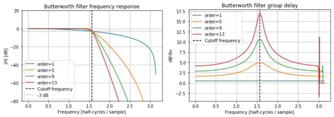
Butterworth filters

• flat response in passband and stopband
• very wide transition band
• higher order = faster transition

1
2

b, a = scipy.signal.butter(N, f_c / f_nyquist)
y = scipy.signal.lfilter(b, a, x)

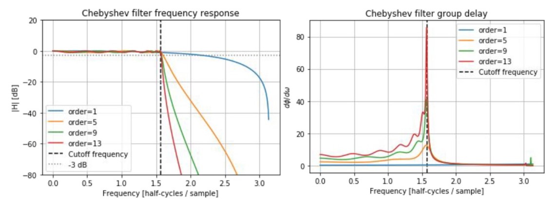
Chebyshev filters

• narrow transition band
• type 1 has passband ripples and flat stopband(pictured); type 2 has stopband ripples and flat passband
• non-linear phase response

1
2

b, a = scipy.signal.cheby1(N, max_ripple, f_c / f_nyquist)
b, a = scipy.signal.cheby2(N, max_ripple, f_c / f_nyquist)

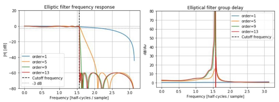
Elliptic filters

• narrowest transition band
• ripples in both passband and stopband
• most non-linear phase response

1

b, a = scipy.signal.ellip(N, max_ripple, min_stop_atten, f_c / f_nyquist)

Z-Transform

$$ X(z) = \sum_{n=0}^{\infty} x[n] \cdot z^{-n} $$

• DFT converts $N$ samples ($x[n]$) into N complex coefficients ($X[m]$)
• z-Transform generalizes the DFT. Specifically, ZT converts $N$ samples ($x[n]$) into a function $X[z]$ on the complex (z-) plane, with $x[n]$ as coefficients of a polynomial in $z^{-1}$. When $z = (e^{j2 \pi \cdot m/N})$, $X(z)$ becomes DFT $X[m]$

Properties

ZT allows us to analyze IIR filters without dependency on signal length N. It has following properties:

• Linearity:
  • $ZT(c_1 \cdot x_1 + c_2 \cdot x_2) = c_1 \cdot ZT(x_1) + c_2 \cdot ZT(x_2)$
• Convolution theorem:
  • $ZT(x * h) = ZT(x) \cdot ZT(h)$
• Shifting theorem:
  • Delaying by $k$ samples $\Leftrightarrow$ $X(z) \rightarrow z^{-k} \cdot X(z)$

Transform function

For a general IIR filter $ y[n] = \sum_{k=0}^K b[k] \cdot x[n-k] - \sum_{k=1}^K a[k] \cdot y[n-k] $, we have $Y(z) = H(z) \cdot X(z)$, where $H(z)$ is the transform function:

$$ H(z) = \dfrac{\sum_{k=0} b[k] \cdot z^{-k}}{1 + \sum_{k=1} a[k] \cdot z^{-k}} $$

Frequency response

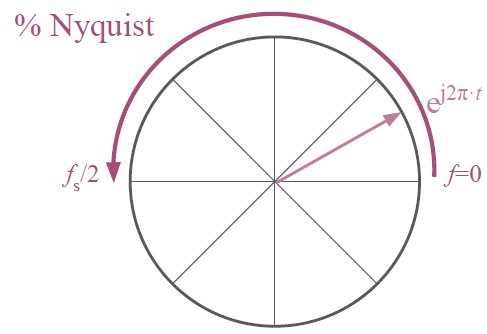
$e^{j2 \pi \cdot m/N}$ is a point on the unit circle in the complex plane, according to IDFT, such a point correpsonds to a sinusoid with frequency $f_s \cdot m/N$, or $ e^{j2 \pi \cdot t} \Rightarrow f_s \cdot t, t \in [0, 1/2]$. Thus, we can relate the angle of points in unit circle with frequencies:

$$ e^{j \theta} \Rightarrow f_s \cdot \theta / 2 \pi $$

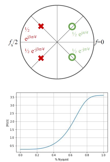
By evaluating the transfer function at $z=e^{2 \pi \cdot t}$ for $t \in [0, 1/2]$, we can see how the frequency magnitude response $|H(e^{j2 \pi \cdot t})|$ changes with frequency $f_s \cdot t$.

Zeros and poles

Places where $H(z) = 0$ are infinitely attenuated and are called zeros of the system. Since $H(z)$ is a polynomial, which is continuous, frequencies near the zeros will also be attenuated. To find zeros, set $\sum b[k] \cdot z^{-k} = 0$ and solve for $z$.

Places where $H(z)$ divides by 0 are called the poles of the system, which correspond to resonance and gain. To find poles, solve for $z$ by denominator $1 + \sum_{k=1} a[k] \cdot z^{-k} = 0$

Given positions of poles and zeros (and total gain), the system is fully determined:

1

[b, a] = scipy.signal.zpk2tf(zeros, poles, gain)

And vice versa:

1

[zeros, poles, gain] = scipy.signal.tf2zpk(b, a)

• If a system has a pole and a zero at the same $z$, they cancel out
• If b and a are real, then poles/zeros always come in conjugate pairs
• A system is stable if all poles are strictly inside the unit circle
• A system is unstable if any poles are strictly outside the unit circle
• Zeros do not affect stability
• Proximity of poles and zeros to the unit circle corresponds to filter sharpness
• Angle $\theta$ of poles and zeros corrspond to frequency ($f_s \cdot \theta / 2 \pi $)